Formal Models for Cryptography
The primary goal of this class is to bring students to a level where they understand enough about cryptography to use it intelligently, while gaining some insight into how cryptographic operations work. However, it is not a cryptography class in the sense of learning the science of cryptography, and the textbook is similarly focused and does not discuss the science of cryptography. The purpose of this handout is to give you some insight into how cryptographers think about security. Even if you never study more cryptography, the concepts that have been developed in cryptography are extremely powerful for the clarity they bring to thinking and reasoning about security.
Some details are glossed over in this handout, and there are subtle issues that are only apparent with more study. If you want to learn more about the formal study of cryptography, I would recommend the book Introduction to Modern Cryptography by Katz and Lindell, or the lecture notes by Bellare and Rogaway (also entitled Introduction to Modern Cryptography!) that are freely available at https://web.cs.ucdavis.edu/~rogaway/classes/227/spring05/book/main.pdf.
The Basics
While you probably have some reasonable intuition about what it means to “break” an encryption scheme or some other cryptographic system, turning this intuition into ideas with enough mathematical rigor to support logical reasoning about security brings up many subtle issues and is quite challenging. One of the great success of cryptographic research in the past few decades has been the development of formal models of security that simultaneously match our intuition of security and provide the logical foundation for rigorous reasoning about security. Any model for security must consider how the adversary is defined, and in this section we discuss three very basic questions that must be answered, related to the adversary’s access, power, and ultimate goal.
What kind of access does the adversary have to the cryptographic system? This is often referred to as the style of attack, and is discussed somewhat in the textbook. While a real-world attack might only have access to captured ciphertext, we primarily consider models in which the adversary is given substantially more power. If we can devise systems that are secure against these powerful attackers, they are certainly secure in other situations in which the adversary is more limited. The two most common adversary models are chosen plaintext attacks and chosen ciphertext attacks. In these models, the adversary is given access to either an encryption device or a device that can decrypt as well as encrypt — picture this device as a tamper-proof piece of hardware that you can feed values (plaintext or ciphertext) into, but the adversary has neither access to nor control over the key that is used. Of course, this is all just an issue of mathematical modeling, not real physical devices, and using terminology from computational complexity theory we refer to these devices as “oracles.”
We also borrow notation from computational complexity theory: we denote the execution of an algorithm \(A\) on inputs \(x\) and \(y\) as \(A(x,y)\), much like in a programming language with function names and parameters. A regular algorithm, like \(A\), can do all the standard computational tasks like arithmetic, logic, looping, control, etc., but what about giving \(A\) access to an oracle such as an encryption oracle? This is not part of a normal computational model, since the encryption oracle computes a function that \(A\) cannot compute on its own (remember, \(A\) does not know the key used by the encryption oracle). One way to view this is that the oracle defines an API (Application Programming Interface), and \(A\) can query the oracle through this API even if it has no ability to compute the oracle function itself. For example, we could denote an encryption oracle by \(\mathcal{E}\), and define the API to be such that \({\mathcal E}\) takes a plaintext value \(p\) and returns a ciphertext value \(c\) (so \(c={\mathcal E}(p)\)). To denote that algorithm \(A\) can use encryption oracle \({\mathcal E}\) when processing inputs \(x\) and \(y\), we provide the oracle name(s) as superscript(s) to the algorithm name, so in this case we write \(A^{\mathcal E}(x,y)\) — this is exactly what we mean by the chosen-plaintext model, where attack algorithm \(A\) has access to an encryption oracle that it can use to encrypt plaintexts of its choosing. If an algorithm has access to multiple oracles then we can give a comma separated list in the superscript, so an algorithm that has access to both encryption and decryption oracles would be written as \(A^{\mathcal{E},\mathcal{D}}(x,y)\) — with access to both encryption and decryption oracles, this is the chosen-ciphertext model.
Example 1a. Lets say that a person is using a block cipher (like AES, but with variable block and key sizes) as a deterministic cipher for small plaintexts: just putting in one block of plaintext and running it through the block cipher directly. The adversary knows that a user is sending a simple “Yes” or “No” message in a ciphertext \(c\), and has access to an encryption oracle. We can define an attack algorithm as follows — notice the superscript on the algorithm name, indicating that the algorithm has access to the encryption oracle, and the use of \({\mathcal E}\) inside the algorithm as a simple function call.
\(A^{\mathcal{E}}(c)\):
if \(\mathcal{E}(\)“Yes”\()=c\) then
return “Yes”
else
return “No”
While the purpose of this example is to show how the oracle concept and notation are used, it’s also a clear example of how a deterministic algorithm with a small set of possible plaintexts can never be secure in the chosen-plaintext model.
What power does the adversary have? It is common in computer science to equate “efficient algorithms” with “polynomial time algorithms” — so algorithms that run in \(O(n)\) time, or \(O(n^2)\) time, or \(O(n^3)\) time are considered efficient, while algorithms that run in \(\Theta(2^n)\) time, \(\Theta(n^n)\) time, \(\Theta(n!)\) time, or even \(\Theta(n^{\log n})\) are not efficient. Since many practical algorithms use randomization (e.g., randomized algorithms for testing primality), we will refer to an algorithm as “efficient” even if it uses randomization, as long as the expected running time of the algorithm is polynomial. The technical term for such an algorithm is a probabilistic polynomial time algorithm.
When we say that there is an efficient attack on a cryptographic system, we mean that there is an efficient algorithm for the adversary that “breaks” the system in some sense (which we’ll consider later). Is it realistic to say that an adversary is an “algorithm”? Can a person use judgments and intuition in breaking a system that can’t be codified in an algorithm? These are more philosophical questions, and the fact is that modern cryptosystems are complex enough that attacks need to be automated in algorithms, so we stick with this idea for our model of security. The one big question that arises from this description is “polynomial in what?” — in other words, what is \(n\) when we say an adversary’s algorithm has running time \(O(n^2)\)? The solution to this in cryptography is that we define algorithms that are parameterized by what we call the “security parameter,” and we denote in this handout with \(\lambda\). In any running time, if we say the adversary runs in time \(O(n^2)\) we mean that it runs in time \(O(\lambda^2)\), where \(\lambda\) is this security parameter. The security parameter might be, for example, the number of bits in a cryptographic key, so that the higher the security parameter the longer the key, and hence (hopefully!) the harder it is to break the system. Our goal then is to create cryptographic algorithms that can be computed efficiently (in time polynomial in \(\lambda\)), but can’t be broken efficiently (i.e., no probabilistic polynomial time algorithm can break the security).
What about calls to the oracle? Since these aren’t standard computational procedures, how long should we say an oracle call takes? In some situations this can be a very important question, and properly accounting for the time an adversary uses in oracle calls is vital. However, in this overview, we only care to distinguish between “polynomial time” and “non-polynomial time”, and a precise accounting isn’t necessary — in fact, we’ll basically ignore the computational time of an oracle call, and just treat it as the amount of time required to write out the parameters to the oracle and to read the result. If you study more cryptography, with a little practice you should get a good feel for when this simplification is appropriate and when it isn’t, but just know that it is appropriate for the discussion in this handout.
Example 1b. We return to Example 1a, and consider the function \(A^{\mathcal E}(c)\) a little further. In particular, this algorithm is precisely the algorithm that would define an adversary operating on a given ciphertext in the chosen-plaintext adversarial model. In the beginning of the example, we said we were dealing with a block cipher that could take on a different block and key sizes. Given the discussion of the current question, hopefully you can see why it was worded this way. Algorithms are analyzed by the time required as the input grows — if the input size if fixed, or has some upper-bound (e.g., AES with keys that cannot be larger than 256 bits), then every algorithm you could possibly run on this, including a brute force attack, is “constant time” or \(O(1)\). Therefore, to make running times meaningful, we need to consider a generalized block cipher in which the key/block size is determined by the security parameter, so we can have a key size of 128 bits, 1024 bits, or even 1,000,000 or more bits.
So what is the time complexity of algorithm \(A^{\mathcal E}(c)\)? The algorithm is about as simple as it could possibly be, with the only time being for preparing the input to \({\mathcal E}\) and checking the result. The plaintext must be padded out to a full block, the size of which is determined by the security parameter, so in the end we see that we would call this a \(O(n)\) time adversary algorithm.
What does it mean for the adversary to “break security”? At first this seems like an obvious question: If we have a secret to protect using encryption, then the adversary breaks security if it learns our secret. This is, in fact, what the adversary does to break the security in Example 1a. However, if we want to establish that a cryptosystem has security in all uses and scenarios, then this is not sufficient. For example, what if we could determine whether the plaintext had some mathematical property — a bit string entering an encryption algorithm can be viewed as a number, so what if we could determine whether that number were even or odd? You might be tempted to say that’s not too bad, but this can cause a problem: if the message were a single word, either “attack” or “retreat”, then it turns out that “attack” is an odd number and “retreat” is an even number, so you just gave away your battle plans! As a general rule, any time you settle for “just a little insecurity” it could and probably will come back and bite you later!
In general then, it seems like our goal should be that the adversary can gain no information whatsoever about the plaintext. Of course, “no information whatsoever” is difficult to define in a rigorous and useful way, but it can be done, and the result is a notion of security that we call semantic security (“semantics” is synonymous with “meaning”, so what we’re really saying is that the adversary gets no meaning from the ciphertext). The notion of semantic security (and the precise definition, which we are avoiding in this handout!) is due to Goldwasser and Micali [S. Goldwasser and S. Micali. “Probabilistic encryption,” Journal of Computer and System Science, Vol. 28, 1984, pp. 270–299] in the early 1980’s, and was one of the breakthrough ideas in defining security for cryptosystems. Goldwasser and Micali won the Turing Award in 2012 largely due to this work, which was the foundation for a long line of successful research rigorously defining security for cryptographic algorithms. Fortunately for us, the difficulty with defining this precisely can be avoided, as we’ll see later with a simpler analysis method that nonetheless gives us this intuitively strong notion of security.
Gaining no information at all seems like about as strong a goal as we can hope for, and it is in fact this goal that is met by the “perfect security” one-time pad system. However, earlier in this class you did an exercise in which you saw that even a one-time pad has a weakness: an attacker, even if she can’t get any information about the plaintext, can modify the ciphertext in such a way that it makes meaningful and predictable changes in the plaintext produced by decrypting the modified ciphertext. As a solution to this problem, Dolev, Dwork, and Naor [D. Dolev, C. Dwork, and M. Naor. “Non-malleable cryptography,” 23rd Symposium on Theory of Computing, 1991, pp. 542–552] defined a security notion that they named “non-malleable security” — essentially, the ciphertext can’t be changed (i.e., isn’t malleable) in a way that could produce a meaningful change to the recovered plaintext. Like semantic security, this is a security notion that intuitively “feels right,” but also like semantic security, rigorously defining this notion is quite tricky (what does a “meaningful change” really mean?). Again, we are saved by other ideas that we will describe later that allow us to achieve this intuitively appealing notion of security while avoiding the messy definition of something being “meaningful.”
So we have seen two important definitions of security that make sense: semantic security and non-malleable security. It turns out that non-malleable security implies semantic security, so it is a strictly stronger notion (i.e., every system that has non-malleable security is also semantically secure). Whether we need the stronger notion depends on what our attack can do, and what the dangers to our system are.
Indistinguishability
The notion of indistinguishability has a long and important history in computer science, and is based on the following philosophical question: If we can’t tell the difference between two objects, are they for all intents and purposes the same? One of the first real uses of this concept is the famous “Turing Test” definition of artificial intelligence described by Alan Turing in 1950: If someone claims to have a program that is truly an artificial intelligence program (has the same intelligence as a person), then consider an experiment in which a person (the interrogator) interacts with either this program (A) or a real person (B) through a chat-like interface, and the chat partner is hidden behind a wall as illustrated below.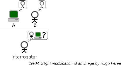
The interrogator can ask the mystery chat partner to describe things any person should know, or reason about things, or analyze a situation, or simply carry on a natural conversation about the weather. If the interrogator truly can’t distinguish between a human and this program, isn’t it natural to say that this program is “thinking” in the same way that a person does?
Or consider another situation in which a human distinguisher is important: lossy compression. Compressing music using the MP3 algorithm can result in a high quality file that is one-fifth or less the size of the best lossless compression, but since it is “lossy” the exact original sound file cannot be reproduced. People who work in lossy compression do human tests in which they play randomly ordered samples, with the original music and the compressed version, to see if people can hear the difference. If the listener can’t distinguish between the two, then does it really matter if some of the original information was lost?
In cryptography, the distinguisher is not a human: we’re interested in whether things are indistinguishable to an adversary, which we defined earlier as a probabilistic polynomial time algorithm. If we have two objects (which could be ciphertexts or something else) for which no probabilistic polynomial time algorithm can tell the difference, then we say these objects are computationally indistinguishable. This turns out to be a very powerful notion, and is the cornerstone of modern cryptographic arguments.
Security Games for Encryption
Returning to the appealing notion of semantic security, recall that this means that the adversary can get no information whatsoever out of a ciphertext. If the adversary could process a ciphertext and determine whether the corresponding plaintext were even or odd, then it could distinguish between encryptions of even and odd values. If it could determine whether the plaintext were a perfect square, it could distinguish between encryptions of squares and non-squares. In fact, if the adversary can get any information at all from the ciphertext, we can view this as a distinguishability problem: For whatever property is being discovered about the plaintext, an adversary could create two plaintexts \(p_0\) and \(p_1\) so that \(p_0\) has the property (i.e., is even, is a perfect square, …) and \(p_1\) does not. Then we ask this: can the adversary distinguish between encryptions of \(p_0\) and \(p_1\)?
Chosen-Plaintext Game and Semantic Security
We first consider the chosen-plaintext model and turn this into a game as follows: the adversary is defined by two different algorithms, both of which have access to an encryption oracle. The adversary operation is divided into two phases: (1) the setup phase is denoted \(A_1^{\mathcal E}(1^\lambda)\) and allows the allows the adversary to make test encryptions and otherwise probe the encryption scheme in order to come up with two plaintexts \(p_0\) and \(p_1\) for which it believes it can distinguish between their ciphertexts, where the only restriction is that \(|p_0|=|p_1|\); and (2) the processing phase, written \(A_2^{\mathcal E}(c)\), where the adversary takes a ciphertext \(c\) that corresponds to one of these plaintexts and processes this to make a guess \(g\in\{0,1\}\) as to which plaintext was encrypted to form \(c\). We allow the adversary to maintain internal state between \(A_1\) and \(A_2\), and there are technical reasons for writing the \(A_1\) parameter as \(1^\lambda\) that follow from our requirement that all adversary algorithms be polynomial time, but these are some of the details that we’re glossing over in this handout.
Based on this description of the game, consider this as two different games, parameterized by a bit \(b\) that determines which plaintext is encrypted. In other words, we actually have two games \(\textsf{CPA-Game}_0\) and \(\textsf{CPA-Game}_1\), and the adversary doesn’t know which it is playing — its goal is to distinguish between these two games and correctly guess which game it is playing. We can formalize all of this into the following game definition.
\(\textsf{CPA-Game}_{b}(\lambda)\):
\((p_0,p_1)\leftarrow A_1^{\mathcal E}(1^{\lambda})\)
\(c\leftarrow {\mathcal E}(p_b)\)
\(g\leftarrow A_2^{\mathcal E}(c)\)
if \(g=b\) then \(A\) wins!
Let’s consider what happens when we pick the bit \(b\) at random, so it has equal probability of being 0 or 1. The question we ask then is: What is the probability that the adversary will win this game? It’s tempting to think that a really bad adversary can’t win, so has probability of winning close to 0. However, that’s not the case: a really bad adversary in facts wins with probability \(\frac{1}{2}\), as we see in the next example.
Example 2. Consider an adversary that picks two random plaintexts for \(p_0\) and \(p_1\) in the setup phase, and then in the processing phase always returns \(g=0\). This simple adversary wins exactly when \(b=0\), and since we pick \(b\) randomly this happens with probability \(\frac{1}{2}\).
It’s tempting to say that we can adjust the selection of \(b\) so that we can make the probability of the adversary winning very small — for example, if we know that the adversary is using the strategy described in Example 2, we could just pick \(b=1\) and then the adversary would always lose. Can we force the adversary to lose for all secure systems? You can answer that question by working through the following exercise.
Question 1. What if the setup is the same as in Example 2 above, but now we do not have to pick \(b\) randomly — we can pick whatever we think would be worst for the adversary’s strategy. Now consider an adversary that simply flips a coin and returns \(g=0\) with probability \(\frac{1}{2}\) and returns \(g=1\) with probability \(\frac{1}{2}\). What is the probability that the adversary wins the game in this situation? Does it matter how we pick \(b\)?
This leads to our final concept: the advantage of an adversary for a particular game. Since our “baseline” winning probability is \(\frac{1}{2}\) we define the advantage of an adversary \(A\) in game \(G\) as the distance to this baseline probability. We denote the advantage of adversary \(A\) for game \(G\) and security parameter \(\lambda\) by \(Adv_{G,A}(\lambda)\), and then the formal definition is
\[Adv_{G,A}(\lambda) = \left| Prob(A\mbox{ wins game }G(\lambda)) - \frac{1}{2} \right| \, . \]
The absolute value is there because we are only interested in how far from \(\frac{1}{2}\) the winning probability is, not whether it is larger or smaller than \(\frac{1}{2}\).
Question 2. It seems like the adversary would really want its winning probability to be greater than \(\frac{1}{2}\) so that it wins more often than just random guessing. However, the absolute value in equation~() destroys the information about whether the adversary wins more than half the time or loses more than half the time. Why doesn’t this matter? (Hint: Can out you turn an adversary that wins with probability less than \(\frac{1}{2}\) into one that wins with probability greater than \(\frac{1}{2}\)?)
Our goal then is to make cryptographic schemes such that the advantage is low for any adversary. The next question to ask is then this: Is it possible for an encryption scheme to not allow any positive advantage at all? You can discover the answer to this in the following question.
Question 3. Consider an encryption scheme that uses \(\lambda\)-bit encryption keys, so the key size is chosen to match the security parameter. Now consider an adversary that does the following: At the beginning of the setup phase, the adversary picks a random key \(k\in\{0,1\}^{\lambda}\) for the encryption scheme, and then does some test encryptions to see whether this key can decrypt the test encryptions properly, verifying whether it matches the key being used by the encryption oracle. After this testing, the adversary picks two random plaintexts \(p_0\) and \(p_1\), and returns the pair \((p_0,p_1)\). For the processing phase, if the key \(k\) passed the tests in the setup phase, then the adversary uses that key to decrypt ciphertext \(c\) and so can pick the correct bit for its guess \(g\). If the random key did not pass the tests in the setup phase, then we let \(g\) be a randomly selected bit with equal probability of being 0 or 1. What is the advantage of this adversary? (Note: There’s a subtle point here about whether a key \(k\) could pass the tests in the setup phase and yet still be different from the key used by the encryption oracle — for the purpose of this question you can ignore this, and assume that whenever \(k\) passes the encryption tests it actually is the same as the oracle’s key.)
While we can’t require that the advantage of our adversary be zero, we do want it to be very small. Similar to the way we consider “polynomial time” to be efficient for algorithms, we also use the polynomial/non-polynomial distinction to define what it means for an adversary to “break” an encryption scheme. In particular, adversary \(A\) breaks a cryptographic scheme in the sense of a game \(G\) if \(Adv_{G,A}(\lambda)\geq\frac{1}{\lambda^c}\) for some constant \(c>0\) and all sufficiently large \(\lambda\). In other words, the advantage is at least the reciprocal of some polynomial.
The opposite of a function (like a probability) that is lower bounded by the reciprocal of a polynomial is the notion of a negligible function: a function \(f(\lambda)\) is negligible if for every constant \(c\geq 1\) there exists an \(n_0\geq 1\) such that \(f(\lambda)<\frac{1}{\lambda^c}\) for all \(\lambda\geq n_0\). Thus, an adversary fails to break an encryption scheme if its advantage in the security game is negligible.
This definition of “breaking security” provides a way to define a secure encryption scheme. In particular, an encryption scheme is secure against chosen-plaintext attacks if there is no probabilistic polynomial time adversary that can break the encryption scheme. Or put another way, the scheme is secure if every probabilistic polynomial time adversary has a negligible advantage in the chosen-plaintext game. In the cryptography literature, this particular definition of security is called “IND-CPA security”, which stands for “indistinguishability under chosen-plaintext attack security.” Let’s look at an example of applying all of these definitions to a real problem.
Example 3. Using these notions of security, we now have a very firm and clear basis to show why ECB mode is not chosen-plaintext secure, and hence should be avoided whenever possible. In particular, consider the following adversary definition:
\(A_1^{\mathcal E}(1^\lambda)\): // Block size \(\lambda\) bits
\(p_0 \leftarrow 0^\lambda\) // A block of 0’s
\(p_1 \leftarrow 1^\lambda\) // A block of all 1’s
return \((p_0,p_1)\)
\(A_2^{\mathcal E}(c)\):
if \(c={\mathcal E}(0^\lambda)\) then
return 0
else
return 1
Since ECB mode is deterministic, the call to the encryption oracle in \({\mathcal E}(0^\lambda)\) will return the same ciphertext \(c\) as the game oracle produced for input to \(A_2\) if and only if the oracle was playing the game with \(b=0\), so the adversary will always win the game! Since the probability that the adversary wins is 1, the advantage of the adversary is \(\frac{1}{2}\), which is clearly a non-negligible probability. Therefore this adversary breaks the security of ECB mode, and shows that ECB mode is not secure against chosen plaintext attacks.
This adversary in fact wins against any deterministic encryption scheme, meaning that no deterministic encryption scheme can be secure against chosen-plaintext attacks! This surprises a lot of people who tend to think of encryption schemes as deterministic: feed in plaintext, and you get the same ciphertext each time (although it looks like incomprehensible gibberish). This observation is the theoretical justification that has led to the way encryption is used in practice: no encryption scheme is typically used in practice without adding some randomization. Block ciphers use modes (like CBC mode) that introduce a random initialization vector (IV), and in-practice use of RSA (which we’ll study later) includes randomized padding techniques such as OAEP.
Question 4. In Example 3, it was shown that ECB mode is insecure with respect to chosen-plaintext attacks using an adversary that made a single call to the encryption oracle. It is actually possible to define an adversary that breaks chosen-plaintext security without using the encryption oracle directly at all! Define such an adversary. (Hint: Make the challenge plaintexts multiple blocks so that you can look for block-to-block patterns in the ciphertext.)
We have seen that any deterministic encryption scheme, including ECB mode for a secure block cipher, cannot be secure against chosen-plaintext attacks. While it’s easy to show that some schemes are not secure, what we really want are positive results: showing that a particular cipher is secure. While there are many such examples, there are no particularly simple examples for symmetric encryption schemes, and the level of these proofs goes beyond the level of these notes.
There is one particularly important thing to know about positive results: other than the one-time pad, there are no known absolute proofs of security — everything is conditional, based on some assumption. For example, you can show that CTR mode with a random starting counter value is IND-CPA secure, assuming that the underlying block cipher is a pseudo-random function. That assumption is defined according to a different cryptographic game (indistinguishability between a truly random and a pseudo-random function), but is an assumption and we don’t know if it is true for any real cipher (except for the stateful one-time pad). Several times in class I have referred to the output of cryptographic functions with the completely non-technical phrase “looks like random gibberish” — a pseudo-random function is the formalization of this notion, where the output doesn’t just look like random gibberish to our eyes (which are easy to fool!), but is indistinguishable from random for any probabilistic polynomial time algorithm. The proof of security for CTR mode using this assumption isn’t too complicated for anyone in this class to follow, but is more involved than what we’ll discuss. If you are interested, you can find the full proof in the Bellare and Rogaway lecture notes that were mentioned at the beginning of this handout — while there may be different versions of these notes, in my copy this is in the “Symmetric Encryption” chapter, Section 4.7, as Theorem 4.7.1 (the proof itself is about 2 pages long, but relies on some other material such as the formal definition of pseudo-random functions).
Why must any positive result be based on an assumption? The reason is tied in to some very fundamental computer science. Recall that the most famous and important unsolved computer science problem today is the \(P\) vs. \(NP\) problem. If you could prove that either \(P=NP\) or \(P\neq NP\) then great fame and fortune would be yours. It turns out that if \(P=NP\) then you can win the chosen-plaintext game for any stateless cipher — if you are familiar with the “guess and check” formulation of the class \(NP\), what we’re doing is guessing the encryption key and checking it using some sample encryptions. So the logical statement here is “if \(P=NP\) then no stateless encryption scheme can be IND-CPA secure,” and so through the logical contrapositive we have the equivalent statement “if there exists a stateless encryption scheme that is IND-CPA secure, then \(P\neq NP\).” Therefore, if you could prove some stateless symmetric cipher were IND-CPA secure, without making any assumptions, then you would have just proved that \(P\neq NP\) — which would be followed by fame, fortune, and a solid place in the history books. The difficulty of such proofs is precisely why all security proofs are based on some assumption.
Relation of the chosen-plaintext game to semantic security. In the first section, we described notions of security that matched our intuition as to what “secure” means. Then in this section, it seems like we’ve gotten side-tracked designing games that make some sense, but don’t have the same level of intuitive appeal. The main benefit of the games are that the definitions are straightforward and they make analysis much more simple than trying to wrestle with the formalities required for semantic security. Now the great news: these two notions are in fact equivalent! In other words, an encryption scheme is semantically secure if and only if it is secure in the chosen-plaintext game. That means we get the intuitively appealing notion of semantic security, while dealing with the much simpler definitions of game-based security.
Chosen-Ciphertext Game and Non-Malleable Security
In the last section we defined a game for chosen-plaintext security. In this section, we consider giving the adversary access to a decryption oracle as well as an encryption oracle, resulting in the chosen-ciphertext game:
\(\textsf{CCA-Game}_{b}(\lambda)\):
\((p_0,p_1)\leftarrow A_1^{\mathcal E,D}(1^{\lambda})\)
\(c\leftarrow {\mathcal E}(p_b)\)
\(g\leftarrow A_2^{\mathcal E,D}(c)\) // Note: \(A_2\) is not permitted to call \({\mathcal D}(c)\)
If \(g=b\) then \(A\) wins!
In addition to adding access to the decryption oracle, there is one complication: If the adversary has unrestricted access to the decryption oracle after the challenge ciphertext \(c\) is known, then the adversary could just decrypt \(c\) and find which of the challenge plaintexts was encrypted. To avoid this obvious problem, we make a simple change: once ciphertext \(c\) has been produced, we simply don’t allow \(A_2\) to call the decryption oracle with this ciphertext. There are no other restrictions on the oracles calls, and all other notions such as advantage are the same as in IND-CPA security. The result is what we call IND-CCA2 security (the “2” isn’t a typo, and is important, but since this handout doesn’t cover the other style of CCA security we don’t need to go into what makes this the second style of CCA security).
Example 4. Consider random-start CTR mode encryption with a generalized block cipher like we used in previous examples (“random-start” means that the counter value for the first block is picked at random). In the last section we mentioned that such a scheme is IND-CPA secure if the underlying block cipher is pseudo-random. To do this style of encryption we first pick a random initialization vector (IV), and then produce a sequence of pseudo-random bit vectors by calling \(R_0=Cipher(IV)\), \(R_1=Cipher(IV+1)\), \(R_2=Cipher(IV+2)\), \(\cdots\) and then computing ciphertext blocks as \(C_0=P_0\oplus R_0\), \(C_1=P_1\oplus R_1\), \(C_2=P_2\oplus R_2\), \(\cdots\). The final ciphertext is then \((IV,C_0,C_1,C_2,\cdots)\). Now define an adversary as follows.
\(A_1^{\mathcal E,D}(1^\lambda)\): // Block size \(\lambda\) bits
\(p_0 \leftarrow 0^\lambda\) // A block of 0’s
\(p_1 \leftarrow 1^\lambda\) // A block of all 1’s
return \((p_0,p_1)\)
\(A_2^{\mathcal E,D}(c)\): // Note: \(c\) is of the form \((IV,C_0)\)
\(c'=(IV,C_0\oplus 0^{\lambda-1}1)\)
\(p'={\mathcal D}(c')\)
if \(p'=0^{\lambda-1}1\) then
return 0
else
return 1
Since \(c'\) differs from \(c\), it doesn’t trigger the restriction on decryption oracle calls. However, all we’ve done is flipped the last bit of the ciphertext — and since decryption just results in the original plaintext with the last bit similarly flipped, we can easily recognize which of the two challenge plaintexts was encrypted. The probability that the adversary wins this game is 1, giving an advantage of \(\frac{1}{2}\). Therefore, CTR mode is not secure with respect to chosen-ciphertext attacks.
Just like IND-CPA security is equivalent to semantic security, it turns out that IND-CCA2 security is equivalent to non-malleable security. Our last example gave some hints about this relationship: we put in a restriction that the decryption oracle is not allowed to call \({\mathcal D}(c)\), but if the encryption scheme is malleable then we can modify \(c\) to produce a related ciphertext \(c'\), for which the associated plaintext \(p'\) is related to \(p\) in a meaningful way. Thus the adversary can “get around” the restriction on the decryption oracle by calling \({\mathcal D}(c')\) to get \(p'\). Since malleability says we know the relation of \(p'\) to \(p\), the adversary can now compute \(p\) and determine which of the challenge plaintexts was encrypted.
Much like IND-CPA security, it is possible to prove that some ciphers are IND-CCA2 secure under certain assumptions, but this is beyond the scope of this handout and our study of formal models in this class. However, the converse is easier: in some cases it is fairly straightforward to identify malleability weaknesses and turn them into a proof that a scheme is not IND-CCA2 secure, as in the following question.
Question 5. Output Feedback (OFB) mode is one of the less-used block cipher modes of operation, and is described briefly in Section 8.1.7 of the textbook. Prove that OFB mode is not IND-CCA2 secure.