Back in 1996, a sequence of numbers known as the Perrin numbers received a lot of attention, due to an article in Scientific American:
Ian Stewart. “Mathematical Recreations: Tales of a Neglected Number”, Scientific American, June 1996, pp. 102-103.
At the time, a group of people on the sci.math Usenet discussion forum (including the author of this summary) decided to try to solve the open problem described in that article: If \(n\) divides \(P(n)\), must \(n\) always be prime? We did in fact answer that question in the negative, finding two counter-examples, but being able to answer the question required both good computers and clever algorithms. While good algorithms must be used, it requires nothing beyond material that should be understandable to any computer science student that has completed an advanced data structures class. Because of this, I have regularly used this as an introduction to my algorithms classes, showing how algorithm design, analysis with recurrence equations, and induction proofs, all come together to solve this problem.
A few years after solving this problem, we discovered that we were not the first. The problem had actually been solved in 1982 (unknown to either us or to Ian Stewart, who wrote the Scientific American article):
William Adams and Daniel Shanks. “Strong primality tests that are not sufficient,” Mathematics of Computation, Vol. 39, pp. 255-300, 1982. DOI 10.2307/2007637
However, it’s still a great problem to use to introduce students to algorithms! This web page is an update to my 1996 presentation, with all the computational tasks run on modern hardware (an Intel Core i7-7700 CPU). This hardware is approximately 200 times faster than the hardware of the original tests, but still would not be fast enough to solve this problem without careful algorithm design.
Perrin numbers are interesting, and provide an excellent real-world example of techniques used in the design and analysis of algorithms, as well as an example of the importance of designing good algorithms. In fact, due to clever (but simple to describe) algorithms, an open question that has been around for almost a century has finally been solved. This is possible in part because of faster computers, but this is not enough — without the efficient algorithm for Perrin number computation, even the fastest computers today would not have been able to solve the problem that we will look at.
Perrin numbers are closely related to Fibonacci numbers, as is clear from the definition of these two sequences:
  Fibonacci Sequence        Perrin Sequence
  ==================        ===============

   F(0)=0                    P(0)=3
   F(1)=1                    P(1)=0
   F(n)=F(n-1)+F(n-2)        P(2)=2
                             P(n)=P(n-2)+P(n-3)
Thus, the first 15 Perrin numbers are
Now do something that at first seems odd. Look at the above list, and make a note of the values of \(n\) such that \(P(n)\) is divisible by \(n\). For example, \(P(2)=2\) is divisible by 2, \(P(3)=3\) is divisible by 3, but \(P(4)=2\) is not divisible by 4. The values of \(n\) which evenly divide \(P(n)\) in the above list are exactly 2, 3, 5, 7, 11, and 13. This list is exactly the list of prime numbers in the range \(0\ldots 14\)! If you keep calculating in this way, you’ll see that the values of \(n\) that evenly divide into \(P(n)\) seem to be exactly the prime numbers. This is fascinating and important because the sequence of prime numbers has no known simple, easily exploitable structure. So the interesting question, which was first asked around 1899, becomes:
Let \(S\) be the set of all numbers \(n\) such that \(P(n)\) is divisible by \(n\). Is \(S\) the set of all prime numbers?
Before long, it was shown that for all prime \(n\), \(P(n)\) is divisible by \(n\). We will use the name “Perrin-positive” for any number \(n\) for which \(P(n)\) is divisible by \(n\).1 By the first sentence of this paragraph, all prime numbers are Perrin-positive, but are all Perrin-positive numbers actually prime numbers? In other words, we are interested in asking “Are there any non-prime (composite) values \(n\) such that \(P(n)\) is divisible by \(n\)?” Looking at relatively small values of \(n\), the answer to this question seems to be “no,” meaning that the set \(S\) appears to consist of exactly the prime numbers. If there are indeed any composite values of \(n\) such that \(P(n)\) is divisible by \(n\), this seems like a perfect job for a computer: find such an \(n\), so that this counter-example can prove that the set \(S\) is not the same as the set of prime numbers. To solve this task, we set out to solve the following problem: write a program that outputs all Perrin-positive numbers from 1 to 1 billion.
The first thing you notice if you start computing Perrin numbers is that they get very big, very fast, and so they exceed the size of an integer variable on the computer (and if you use software that lets you deal with such big numbers, the computations get very slow). How can we correct this?
We’re really just interested in whether \(P(n)\) is divisible by \(n\). In other words: Is (\(P(n)\bmod n\)) equal to zero? It’s a basic fact of mathematics that if you’re interested in computing (\(f(n)\bmod m\)), and the computation of \(f(n)\) involves only simple operations (like additions, subtractions, and multiplications), then you can use the mod operation at any time during the computation in order to keep the values small. For example, if we use \(P(n,m)\) to denote (\(P(n)\bmod m\)) we can use the following formulas for computing \(P(n,m)\):
        P(0,m)=3 mod m
        P(1,m)=0
        P(2,m)=2 mod m
        P(n,m)=(P(n-2,m)+P(n-3,m)) mod m
Now we can compute \(P(n,n)\). Notice that \(P(n)\) is divisible by \(n\) if and only if \(P(n,n)=0\). Furthermore, by directly using these formulas when computing \(P(n,n)\), no intermediate value will ever be larger than \(2n\). This means that if you’re interested in \(P(n)\) for \(n=\) 1,000,000,000, then no intermediate value will ever be larger than 2,000,000,000, which fits in a 32-bit signed integer, and so we can actually make this computation.
Now the question of algorithms arises. The first thought is to take the formulas above, and implement them directly using a recursive algorithm. It is a simple matter to make a C++ implementation of this method, and use it to check out small values of \(n\). The values of \(P(n)\bmod n\) can be summarized in a table, which shows that for small values of \(n\), no composite number \(n\) evenly divides \(P(n)\).
The problem is that when \(n\) starts getting larger, this program takes a very long time to run. Why? This is where the analysis of algorithms comes in handy. Since this algorithm is recursive, we will describe the running time of the algorithm with a recurrence equation:
\[ T(n) = \left\{ \begin{array}{ll} T(n-2)+T(n-3)+c_2 ,& \mbox{for }n\geq 3;\\ c_1 ,& \mbox{for }n<3 \end{array}\right. \]
For people who know that the Fibonacci sequence grows exponentially fast, it should be no surprise that the function \(T(n)\) also grows exponentially fast. In fact, we will show here that \(T(n)\) is greater than \(c\cdot (1.3)^n\) for the constant \(c=c_1/(1.3)^3\) and all non-negative \(n\). The proof of this fact is by induction:
- Base:
- It is easy to verify that \(T(n) >c\cdot (1.3)^n\) for n=0, 1, and 2.
- Induction:
- Assume that \(T(k) > c\cdot (1.3)^k\) for \(k<n\). Then we can derive: \[ \begin{align} T(n) &= T(n-2) + T(n-3) + c_2\\ &> c\cdot (1.3)^{n-2} + c\cdot (1.3)^{n-3} + c_2 \mbox{ (by ind. hyp.)}\\ &= (1.3\cdot c+c)\cdot (1.3)^{n-3} + c_2\\ &= \frac{2.3}{1.3^3} \cdot c \cdot (1.3)^n + c_2\\ &> 1.04 \cdot c \cdot (1.3)^n + c_2\\ &> c \cdot (1.3)^n \end{align} \] This completes the proof.
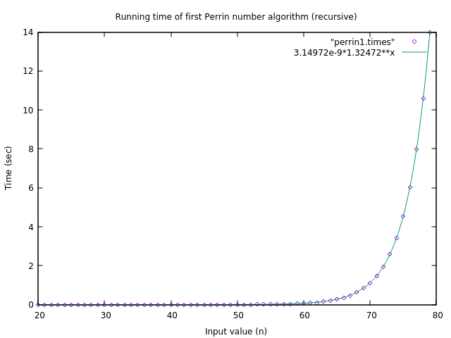
Using asymptotic notation, we can say that the running time of this algorithm is \(\Omega((1.3)^n)\), which shows that the running time of the algorithm grows exponentially with \(n\). A slightly more involved analysis shows that the running time actually grows at a rate that is closer to \((1.325)^n\), and so we can plot actual data points of this implementation’s running time with the best curve fit of \(c\cdot (1.325)^n\). This plot shows that the data points to fit very nicely with this curve, and so this is an accurate estimate of the running time.
What does this tell us? Let’s say you want to compute \(P(n)\bmod n\) for \(n=150\). That’s still a very small value of \(n\), and yet our formula tells us that this would take approximately 207 years just to compute this one Perrin value! Since we can’t even compute the one value of (\(P(150)\bmod 150\)) in under a hundred years, the amount of time it takes to compute the Perrin-positive numbers in the range 1..1 billion is simply incomprehensibly large. We clearly need to do better.
Why is the last implementation so slow? If you start writing down the values computed, you will soon realize that this algorithm repeats its work over and over again. In particular, to compute \(P(n)\) the algorithm recursively computes \(P(n-2)\) and \(P(n-3)\), and these two recursive calls make further recursive calls to compute \(P(n-4)\), \(P(n-5)\), \(P(n-5)\), and \(P(n-6)\). Notice that \(P(n-5)\) is listed twice. That’s not a typo; the algorithm actually computes \(P(n-5)\) twice. Clearly this is inefficient.
The solution is to remember the values that you have computed, and don’t compute any particular value more than once. When this is done, and values are computed from the bottom up, this is known as dynamic programming, which is a very powerful algorithmic technique. Despite the simplicity of this particular algorithm, dynamic programming is full of small difficulties, and is a topic that students find very difficult to understand. Remember the name “dynamic programming,” and we’ll get back to it in depth later in the course.
For this particular problem, the only time we need to know a value \(P(k)\) is when we are computing \(P(k+2)\) and \(P(k+3)\). So if we compute the values in increasing order, remembering the last 3 values in the sequence, we can easily compute the Perrin sequence. The C++ implementation of this is not difficult, and since it simply iterates up to \(n\), with a constant amount of work per iteration, it should be clear that the running time of this algorithm is \(Theta(n)\). So we’ve gone from an exponential time algorithm to a linear time algorithm! This is excellent progress.
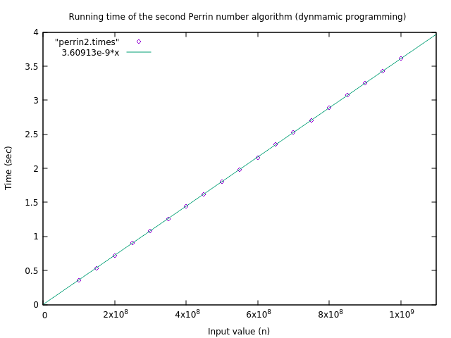
We can again time this algorithm and fit a linear function to it, giving a plot that shows the running time behavior of this algorithm. Computing (\(P(n)\bmod n\)) for \(n=150\) went from taking 207 years for the last algorithm, to only about 0.54 microseconds for this algorithm. That’s a pretty good improvement, and shows why exponential time algorithms are really, really bad. However, avoid the false conclusion that recursion is bad — there are situations where recursion is a very fast, efficient, and clean way of solving a problem. We’ll see several examples of this later in the course.
In fact, computing (\(P(n)\bmod n\)) for \(n=\) 1,000,000,000 takes around 3.6 seconds, so can we solve our problem of listing all Perrin-positive numbers in the range 1 to 1 billion now? Since the running time of this latest, relatively efficient algorithm is a linear function, we can add up the running time over all input sizes using the standard arithmetic sum formula. We see that the time required would be… about 57 years. Oops. We still have a big problem.
Are we stuck? It seems like we might be, since computing \(P(n)\) seems to require computing \(P(n-2)\) which seems to require computing \(P(n-4)\) and so on. So how could you possibly do better than linear time? Well, the fact of the matter is that for any linear recurrence such as Perrin numbers or Fibonacci numbers, you can compute the \(n\)th value in only \(O(\log n)\) time. This seems impossible at first, but illustrates the value of reducing a problem to a different problem, and then applying an efficient algorithm for that problem. Let’s see what that means.
Remembering how to multiply a matrix times a vector, we see that for any value \(n>1\) we can write the following linear algebra equation that represents one iteration of the last algorithm:
\[ \left[\begin{array}{ccc} 0 & 1 & 1 \\ 1 & 0 & 0 \\ 0 & 1 & 0 \end{array}\right] \left[\begin{array}{c} P(n-1) \\ P(n-2) \\ P(n-3) \end{array}\right] = \left[\begin{array}{c} P(n-2)+P(n-3) \\ P(n-1) \\ P(n-2) \end{array}\right] = \left[\begin{array}{c} P(n) \\ P(n-1) \\ P(n-2) \end{array}\right] \]
Now, of course, this whole expression can be multiplied by the same matrix to get a vector containing \(P(n-1)\), \(P(n)\), and \(P(n+1)\). Extending this argument, if M represents the matrix in the above expression, and V represents the vector of initial values: \([2, 0, 3]^T\), then we by computing the \((n-2)\)nd power of the matrix M we can compute:
\[ M^{n-2}\cdot V = \left[\begin{array}{c} P(n) \\ P(n-1) \\ P(n-2) \end{array}\right] \]
So now, in order to compute the \(n\)th Perrin number, we simply need to raise a 3x3 matrix to a power. This process is called a “reduction,” and we can say that we have “reduced the problem of computing the \(n\)th Perrin number to the problem of computing the \(n\)th power of a 3x3 matrix.”
Why is this a good thing? While not many people have spent a great deal of time trying to come up with efficient algorithms for the rather esoteric problem of computing Perrin numbers, there has been a great deal of work on algorithms for very fundamental problems, such as raising a matrix to a power. Now we can use those algorithm in order to solve our problem for Perrin numbers.
If you’re interested in computing \(M^{16}\), one way to do this would be to multiply \(M\) by itself 16 times. This is essentially what our last algorithm did when computing Perrin numbers. Alternatively, we could square \(M\), square the result, square that result, and finally square that result. This computes \((((M^2)^2)^2)^2 = M^{16}\) using only four matrix multiplies rather than the 16 that the naive method uses. For any value of \(n\) that is a power of two, we can use this exact method to compute \(M^n\) by using only \(\log_2 n\) matrix multiplications. This can, in fact, be generalized to powers \(n\) that are not powers of two, and this is fairly easily implemented in C++ as an operation on a class of 3x3 matrices.
Next, we use this 3x3 matrix class in order to compute Perrin numbers in this new C++ implementation. By the above discussion, we have now reduced the time to \(O(\log n)\). However, the program got much more complicated, and it’s expected that the constant factor that the big-oh notation ignores must be fairly large compared to the last algorithms. So is this really an improvement?
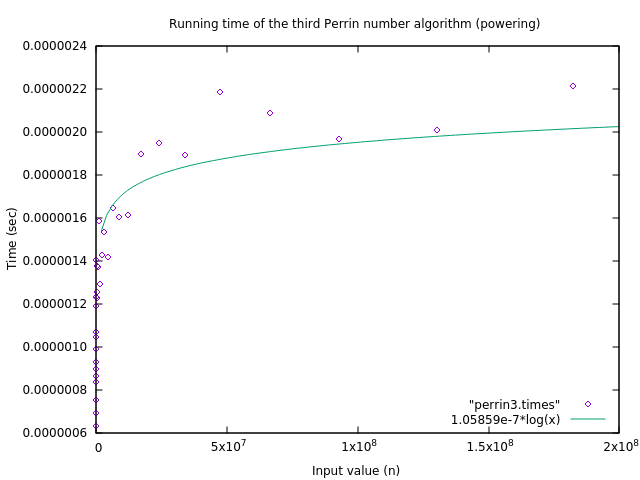
This implementation was timed when computing (\(P(n)\bmod n\)) for \(n=\) 1 billion, and it took only about 2.2 microseconds to compute. Compare this to the 3.6 seconds of the last implementation, which seemed so good at the time! While the running time of this algorithm is slightly more chaotic than that of the previous implementations, we can still fit a function of the form \(c\cdot \log n\) to it and plot the results.
The final question to ask is, how long will this algorithm take to compute all Perrin-positive numbers from 1 to 1 billion? Using our formula for the running time, we can estimate that it will take around 35 minutes. This is clearly an amount of time that we can deal with! (Note: On the original computer we used, in 1996, this calculation took 7 days – a lot longer, but still manageable!)
Now we’ve got an algorithm that solves our problem in a reasonable amount of time. What does it tell us about our open question? It turns out that there are Perrin-positive numbers that are in fact composite numbers. However, the only two such numbers less than a million are 271,441 and 904,631. So apparently these counter-examples to the primality of Perrin-positive numbers are exceedingly rare. While this gives a very clear answer to the question posed at the beginning, it’s still an astounding property that there are so few composite Perrin pseudo-primes.
Note that in my original presentation/write-up, I used the term “Perrin pseudoprime” for what I am now calling “Perrin-positive.” While “pseudoprime” is sometimes used in this context, it more commonly refers to values which pass a test but are in fact composite (in other words, just the counter-examples we are looking for). I have changed the terminology here to match this more common usage.↩